Inelastic Bayes Fitting

Overview

Provides Bayesian analysis routines primarily for use with QENS data.

Action Buttons

Settings

Opens the Settings GUI which allows you to customize the settings for the Indirect interfaces.

?

Opens this help page.

Backend selection box

This drop down selects whether to use the quasielasticbayes or quickbayes package as the underlying model for the Quasi and Stretch tabs.

Backend selected	Underlying algorithms
quasielasticbayes	BayesQuasi & BayesStretch
quickbayes	BayesQuasi2 & BayesStretch2

Manage Directories

Opens the Manage Directories dialog allowing you to change your search directories and default save directory and enable/disable data archive search.

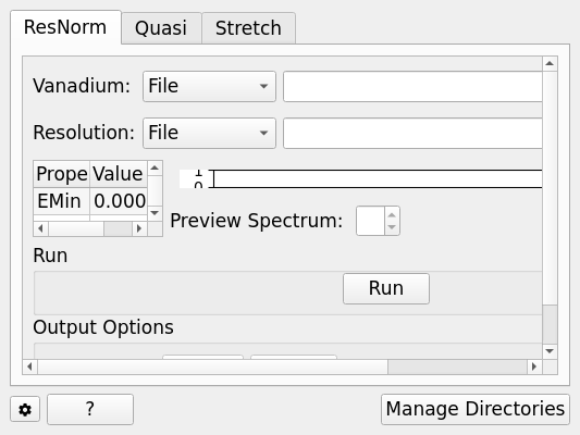
ResNorm

This tab creates a group ‘normalisation’ file by taking a resolution file and fitting it to all the groups in the resolution (vanadium) data file which has the same grouping as the sample data of interest.

The routine fits the width of the resolution file to give a ‘stretch factor’ and the area provides an intensity normalisation factor.

The fitted parameters are in the group workspace with suffix _ResNorm with additional suffices of _Intensity & _Stretch.

The processing on this tab is provided by the ResNorm algorithm.

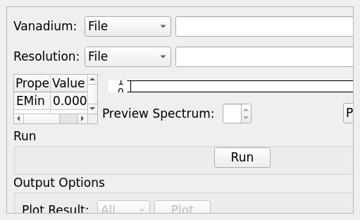
Options

Parameter	Description
Vanadium File	Either a reduced file created using the Energy Transfer tab or a \(S(Q, \omega)\) file
Resolution File	A resolution file created using the Calibration Tab
Plot Current Preview	Plots the currently selected preview plot in a separate external window
EMin & EMax	The energy range to perform fitting within
Preview Spectrum	Changes the spectrum displayed in the preview plot
Run	Runs the processing configured on the current tab
Plot	Plots the selected parameter stored in the result workspaces
Save Result	Saves the result in the default save directory

Quasi

The model that is being fitted is that of a \(\delta\)-function (elastic component) of amplitude \(A(0)\) and Lorentzians of amplitude \(A(j)\) and HWHM \(W(j)\) where \(j=1,2,3\). The whole function is then convolved with the resolution function. The -function and Lorentzians are intrinsically normalised to unity so that the amplitudes represent their integrated areas.

For a Lorentzian, the Fourier transform does the conversion: \(1/(x^{2}+\delta^{2}) \Leftrightarrow exp[-2\pi(\delta k)]\). If \(x\) is identified with energy \(E\) and \(2\pi k\) with \(t/\hbar\) where t is time then: \(1/[E^{2}+(\hbar / \tau)^{2}] \Leftrightarrow exp[-t /\tau]\) and \(\sigma\) is identified with \(\hbar / \tau\). The program estimates the quasielastic components of each of the groups of spectra and requires the resolution file and optionally the normalisation file created by ResNorm.

For a Stretched Exponential, the choice of several Lorentzians is replaced with a single function with the shape : \(\psi\beta(x) \Leftrightarrow exp[-2\pi(\sigma k)\beta]\). This, in the energy to time FT transformation, is \(\psi\beta(E) \Leftrightarrow exp[-(t/\tau)\beta]\). So \(\sigma\) is identified with \((2\pi)\beta\hbar/\tau\) . The model that is fitted is that of an elastic component and the stretched exponential and the program gives the best estimate for the \(\beta\) parameter and the width for each group of spectra.

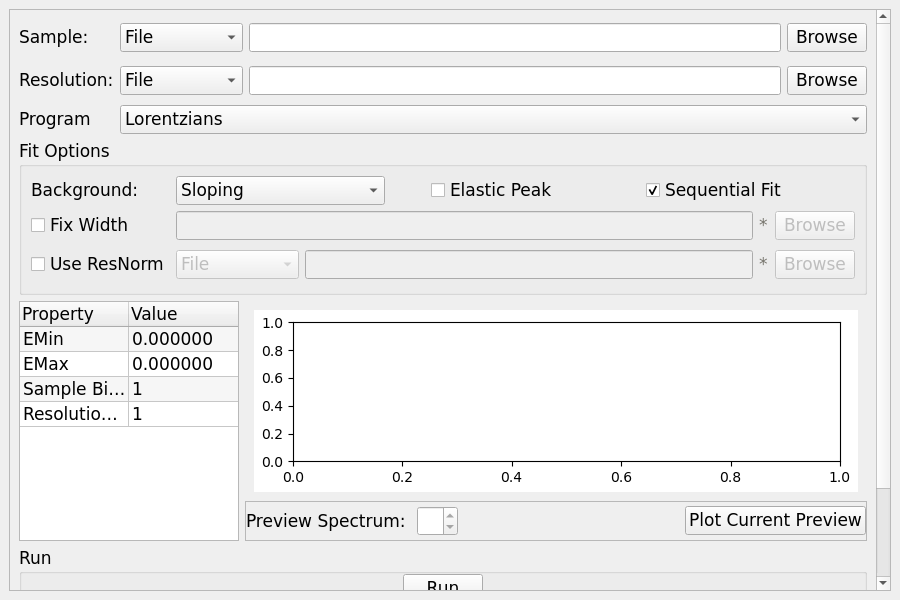
Options

Parameter	Description
Sample	Either a reduced file created using the Energy tab or a \(S(Q, \omega)\) file.
Resolution	A resolution file created using the Calibration Tab
Program	The curve fitting program to use
Background	The background fitting program to use
Elastic Peak	If an elastic peak should be used
Sequential Fit	Enabled multiple fitting iterations
Plot Current Preview	Plots the currently selected preview plot in a separate external window
Fix Width	Allows selection of a width file
Use ResNorm	Allows selection of a ResNorm output file or workspace to use with fitting
EMin & EMax	The energy range to perform fitting within
Sample Binning	Sample binning to use
Resolution Binning	Resolution binning to use
Preview Spectrum	Changes the spectrum displayed in the preview plot
Run	Runs the processing configured on the current tab
Plot	Plots the selected parameter stored in the result workspaces
Save Result	Saves the result in the default save directory

Stretch

This is a variation of the stretched exponential option of Quasi. For each spectrum, a fit is performed for a grid of β and σ values. The distribution of goodness of fit values is plotted. Some of the options change depending on the underlying model selected.

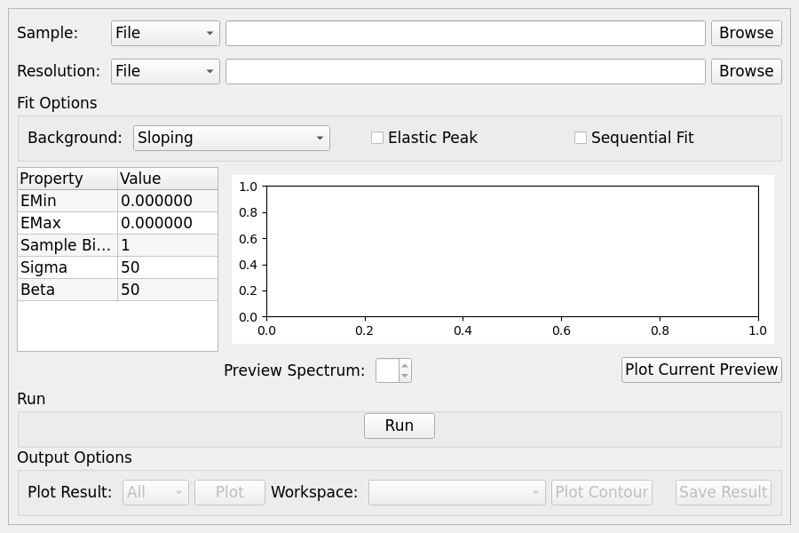
Options

There are some parameters exclusive of either quasielasticbayes or quickbayes model that change automatically depending on the backend selection. For both models:

Parameter	Description
Sample	Either a reduced file created using the Energy tab or a \(S(Q, \omega)\) file.
Resolution	A resolution file created using the Calibration Tab
Background	The background fitting program to use
Elastic Peak	If an elastic peak should be used
EMin & EMax	The energy range to perform fitting within
Sigma	Number of Sigma(FWHM) values
Beta	Number of Beta values
Plot Current Preview	Plots the currently selected preview plot in a separate external window
Preview Spectrum	Changes the spectrum displayed in the preview plot
Run	Runs the processing configured on the current tab
Plot	Plots the selected parameter stored in the result workspaces
Plot Contour	Produces a contour plot of the selected workspaces
Save Result	Saves the result in the default save directory

For quasielastic model there are also the following parameters:

Sequential Fit	Enabled multiple fitting iterations
Sample Binning	Sample binning to use

While for quickbayes the additional parameters are:

Start Beta	Initial value of Beta
End Beta	Final value of Beta
Start Sigma	Initial value of Sigma(FWHM)
End Sigma	Final value of Sigma(FWHM)

Categories: Interfaces | Inelastic